Speedup the Binary Search

Introduction

Binary search is known as the fastest search algorithm on a sorted array. Though it works pretty good in most cases, the performance under some special cases is not favorable. For example, when the size of each element is very big, and there are millions of elements. A single binary search execution need at least 20 times to locate an element. What is even worse, since the size of element is very big, the algorithm cannot utilize the cache to speed up the memory access. Therefore, how to speed up the binary search is the problem I want to talk here.

Simple Analysis

Here is a C implementation of binary search, from where we can understand how binary search shrink the size of range that covers the object value key.

1
2
3
4
5
6
7
8
9
10
11
12
13
14

int BinSearch(int *arr,int len,int key){
    int low=0,high=len-1,mid=0;
    while(low <= high) {
        mid=(low+high)/2;
        if( arr[mid] > key) {
            high=mid-1;
        } else if( arr[mid] < key) {
            low=mid+1;
        } else {
            return mid;
        }
    }
    return -1;
}

As we can see, the binary search shrink the size of range in each iteration by calculating the value mid and divide the range into two equally sized subranges. Therefore, after split $ log_2(n) $ times, binary search can locate a certain element and it is very fast in practice. However, when the sorted data have some degree of features, the strategy that binary search employed to calculate the mid is too conservative.

Guided Binary Search

In this section, I want to optimize the binary search algorithm under the assumption that the data is near uniform. Actually, when the number of elements becomes larger and larger, the data tend to be uniform. The key idea is to estimate the position of the target element and shrink the range as much as possible. Since the speed of binary search is quite fast, the estimate should not be too complex. Here we use a simple but effective idea to estimate the position of the target element.

Suppose we have a sorted array which consists of $N$ elements $ \lbrace e_i | i=1..N \rbrace $. If we want to search an element $t$ in the sorted array, we can use a simple idea to estimate the position of this element. With the assumption that the data is near uniform. For any sorted array, we can assume that

$$ \frac{offset}{L} = \frac{target - min}{max - min} $$

where, $offset$ the distance between target value and minimum value (the first element), $L$ is the length of the array, $target$ is the element we want to search. Therefore, for the first estimation, we have $ L = N $, $max = e_N$, $min = e_1$ and $startPos = 0$. That is

$$ pos = offset +startPos = N \times \frac{t-e_1}{e_N - e_1} $$

Once we obtained the value $v$ of the element at $pos$, we can compare it with $t$, and we have:

1. $t > v$ indicates that the $ pos $ is smaller than the real position $ pos_r $ and we should search the right part of the array
2. $t < v$ indicates that the $ pos $ is bigger than the real position $ pos_r $ and we should search the left part of the array
3. $t = v$ indicates that we find the value and we can directly return the position to caller.

Considering the condition that $t > v$ and we should search the right part of the array. This time, we have $L = N - pos$, $max = e_n$, $min = e_{pos}$ and $startPos = pos$. The estimate position of $t$ can be calculated as follows:

$$ newpos = (N - pos) \times \frac{t - e_{pos}} {e_N - e_{pos} } + pos $$

Also, there are three possible condition listed above. For condition 3, we are lucky and it is trivial. For condition 2, we know that $ pos < pos_r < newpos $. In others words, by estimating the position of $t$ two times, we obtain a new range $(pos,newpos)$ that covers the target value. More importantly, this range is much smaller that one fourth of the original range in practice (see the simulation experiment section). After that, we can use some strategy like directly employ binary search on the new range or continue estimate the position until the length of the new range is less than a given threshold. Experimental results show that the performance are far better than native binary search.

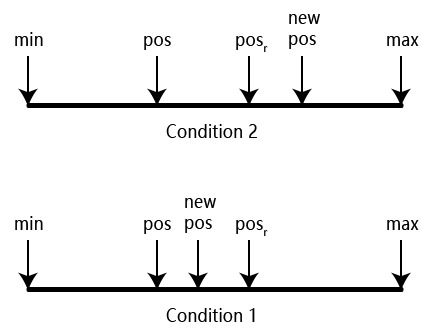
For condition 1, afte two times estimation. The search range now becomes $(newpos,max)$, which is usually larger than one fourth of the original range. To overcome this issue, we can add a offset to force the $newpos$ move to another side of the $pos_r$. Based on this idea, we set the offset to be $\alpha \times (newpos - pos)$, where $\alpha$ is a parameter to control the size of offset.

Implementation in Python

Here is an sample implementation in Python. For the ease of clarity, the estimation logic is represented as a single function. And the strategy used here is to use native binary search after estimating the position two times.

1
2
3
4
5
6
7
8
9
10
11
12
13
14
15
16
17
18
19
20
21
22
23
24
25
26
27
28
29
30
31
32
33
34
35
36
37
38
39
40
41
42
43
44
45
46
47
48
49
50
51
52
53
54
55

def estimate_element_position(data,target,low,high):
    # omit the parameter check
    # since it will not exposed to user
    minVal = data[low]
    maxVal = data[high]
    if (target <= minVal):
        return low
    elif(target >= maxVal):
        return high
    else: # epos must between (low,high)
        epos = low + (high - low) * float(target - minVal)/(maxVal - minVal)
        return int(epos)

def guided_binary_search(data,target,alpha):
    # data is a list
    # target is value user want to search in the list
    # check the parameter
    if (data  == []):
        print "Invalid Input"
        return -1
    elemNum = len(data)
    low = 0
    high = elemNum - 1
    loop_counter = 0
    while (low <= high):
        if (loop_counter == 0):
            # estimate the postion for the first time
            mid = estimate_element_position(data,target,low,high)
        elif(loop_counter == 1):
            # estimate the postion for the second time
            newMid = estimate_element_position(data,target,low,high)
            # add a offset to this new estimation position
            mid = int (newMid + (newMid-mid)*alpha)
            # dut to the offset, mid may bigger than high
            if (mid > high):
                mid = high
            if (mid < low):
                mid = low

        else:
            # after est imated the position two times
            # use binary search strategy
            mid = low + ( (high-low)>>1 )

        loop_counter += 1
        if (data[mid] < target):
            low = mid+1
        elif (data[mid] > target) :
            high = mid-1
        else:
            return mid
    # not find
    return -1

Since we have talked about the theory and implementation of guided binary search, it is time to talk the performance.

Experimental Results

In this section, I will show you the performance analysis of guided binary search. In other words, we need to clarity the following two aspects:

1. What is the possibility that the target is in the range $(pos,newpos)$ after two estimations ?
2. What is the length of range $(pos,newpos)$ after two estimations ?

To answer the above two questions, I conducted a simulation experiment where the data are generated by random generator. You can download the code at Github.

In the simulation experiment, we randomly generate 1 million ($2^{20}$) integers and sort them in an ascending order. After that, we search each element once. Note that for target that are less than the minimum or bigger than the maximum, guided binary search can return in two loops, which is much faster than native binary search, which need 20 comparisons. The following table reports the statistical information.

From the table, we can see that, as the value of $ \alpha $ changes from 0 to 1, the Average Range Length rises and possibility also increases. Also, there is a leap of the possibility from 0.5 to 0.9, which indicates that the added offset is very useful.

What is more, compared with native binary search which needs 20 times of comparisons to locate an element, the guided binary search only need 10 comparisons on average. This means that We need only half of the time of native binary search to locate an element, which is very efficient in practice.

• ← Previous Post
• Next Post →