
In this article, I present a comprehensive literature review of existing research works on Offline Policy Evaluation (OPE). I have incorperated a lot of understandings and interpretations of existing methods that can help you better understand the theory behind. OPE is very useful for estimating the business KPIs such as click rate, it sits between the offline model development and online A/B test, aims to solve the problem of inconsistent evaluation metric between offline development and online deployment.
The draft of this article is completed during my 2023 summer intern at Wayfair.
Tutorials
These tutorials are very similar and are good places to start, it covers latest researches up to 2022.
RecSys2021 Tutorial : slides, codes, video included as well!
KDD2022 Tutorial: slides, codes included (Includes the introduction of the new MIPS estimator) (Highly Recommended!).
RecSys 2022: slides only.
List of Papers
Here are some related papers I found (with a focus on recent publications and model-free methods ).
Off-Policy Evaluation for Large Action Spaces via Embeddings (Feb 2022) : introduces the Marginal IPS (MIPS) estimator.
Off-Policy Evaluation for Large Action Spaces via Conjunct Effect Modeling (May 2023) : introduces the OffCEM estimator.
Contextual Bandits with Large Action Spaces: Made Practical (Jul 2022) : this paper discuss a new type of estimator for OPE with continuous and linear structured action space. NOT so align with our current interest.
Learning Action Embeddings for Off-Policy Evaluation (May 2023) : MIPS estimators requires the action embed data, which may not be available in practice. This paper improve MIPS estimator by learning the action embeddings from data.
Open Bandit Dataset and Pipeline: Towards Realistic and Reproducible Off-Policy Evaluation (Aug. 2020): the open bandit pipeline for evaluating the estimators.
Recap: Designing a more Efficient Estimator for Off-policy Evaluation in Bandits with Large Action Spaces (2019): introduce the recap estimator, it estimates the importance weight via the reciprocal rank of the logged action according to the scores assigned by the new policy. It is also less sensitive to large action space as well. CURRENTLY IMPLEMENTED in ranker-eva library.
Offline Policy Evaluation in Large Action Spaces via Outcome-Oriented Action Grouping (Apr 2023) : improve the large action space evaluation performance by grouping actions.
Policy-Adaptive Estimator Selection for Off-Policy Evaluation (Nov 2022): Introduce a new way to select the best estimator using logged data only, may be useful for meta-evaluation.
Doubly robust off-policy evaluation with shrinkage (Sep 2020) : Introduced a way to estimate the bias of DRos estimator using logging data and true evaluation policy and logging policy. (The formula is on top of the page 17.)
Subgaussian and Differentiable Importance Sampling for Off-Policy Evaluation and Learning (Year 2021): introduced the Sub-Gaussian IPS estimator through Power-Mean Correction of importance sampling.
Balanced off-policy evaluation in general action spaces (Jun 2019): Introduced the Balanced-OPE estimator, it changes the vanilla importance weight in IPS using the output from a trained model to distinguish between logging policy and new policy given context and action pair.
A complete list of papers related to offline reinforcement learning (Topics about OPE also included)
The OPE Problem
Offline Policy Evaluation (OPE) aims to estimate the performance of new stochastic (deterministic policy is just a special case) policy $\pi(a|x)$, given the logging data ${x_i, a_i, r_i}$ generated by logging policy $\pi_0(a|x)$. It avoids the costly and time-consuming A/B test process and thus can creates great business value.
Data Generation Process
Formally, the data is assume to be generated by policy $\pi_0$ with the following procedure.
- we observe some contextual information $x_i \sim p(x)$, where distribution $p$ is unknown to us.
- the policy $\pi_0$ take an action $a_i \sim \pi_0(a|x)$, this is what we can control.
- we observe a reward $r_i \sim q(r|x,a)$, $q$ is also unknown.
The whole logging data ${x_i, a_i, r_i}$ can be treated as samples generated from the joint distribution $p(x) \pi_0(a|x) q(r|x,a)$. One important note here is that we only observe the reward for the action we take.
For example, let’s consider a case of treating heart attacks (image from kdd2022 tutorial). When a patient comes (the context $x$), we can have different treatments (the action $a$), and we can observe the result that whether the treatment is successful (the reward $r$).
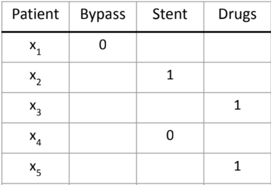
As you can see from above table, we don’t know the outcome of having Drug treatment for patient $x_1$ and so are the other cases.
Policy Value
At the end of the day, what we care in business is the value of a policy, or mathematically the expected reward we can get, which can be formulated as
$$V(\pi_0) = E_{p(x) \pi_0(a|x) q(r|x,a)}[r]$$
This can be estimated easily and accurately (provided with the large amount of logging data) using Monte-Carlo method as
$$ \frac{1}{n} \sum_i r_i $$
This is actually what A/B testing is doing. We put our policy online and gathering the logging of the policy and then we can estimate the business KPI such as click rate ($r_i$ here is binary 0/1).
Goal
Our goal is here to estimate the expect reward we would have if we deploy policy $\pi$ instead of $\pi_0$ using just the logging data, which can be formulated as
$$V(\pi) = E_{p(x) \pi(a|x) q(r|x,a)}[r]$$
where $V(\pi)$ denotes the value of policy $\pi$. It is not immediately clear how to estimate this, because we don’t have the logging data from the new policy $\pi$.
Challenges
The existing estimators such as IPS, SNIPS can have very high variance and bias in practice when the number of actions is large.
How can we develop a good evaluation metric that is accurate in the case of large action space is very challenging and important.
OPE for Ranking System
The above definition of OPE works for both ranking system (where the action is ordered list of actions from the whole action space, the reward in this case will be also be vector) as well traditional recommendation system (where we choose only one action from the whole space, both action and reward is a scalar in this case).
That being said, the following sections mainly focus on the case of single action. But all methods can be adapted into ranking system as well (especially when independence assumption is used)
When conducting OPE for ranking system, we usually have assumptions on how customers interactive the ranking system (called user behavior model).
independence, this basically means the customer interact with recommend list of items independently, i.e. whether the customer will click the item (action) only depends on the customer (context) and the item itself.
cascade, which is quite popular in research community now. It assumes customer interact with the recommend items one-by-one, from position 1 to position n. In this case, whether the customer will click the item at position $i$ only depends on the customer (context) and all the previous item $j = {1,…,i-1}$.
For more information regard the OPE in ranking systems, you can refer to the KDD 2022 Tutorial (at least a good start point). For all future contents, I will mainly focuses on single action recommendation system.
Summary of Classical Estimators
It is always good to see how the classical estimators work. This is also what most existing works based on.
Preliminary
We usually consider the following properties of an estimators.
- Bias
- Variance
- Hyperparameters
- Stableness
- Running time
- Extra Assumptions
The existing estimators can be roughly divided into three categories:
- model based method, such as Direct Method (DM) and its variants.
- model free method, such as Inverse Propensity Score (IPS) and its variants.
- the hybrid of above two, or called hybrid methods, such as Doubly Robust (DR) and its variants.
I will go over these three baseline methods first and then some latest estimators that are improved version of these 3 baseline estimators.
Direct Method (DM)
This is perhaps the most intuitive method, recalled that the OPE is in general hard because we only observe the reward of the action we take. If we can somehow know the rewards of all actions we take, estimating the reward for new policy would be very easy.
In direct method, the idea is impute these missing values (the reward that is not observed) by training a reward model $\widehat r$, such that $r_i = \widehat r (x_i, a_i)$.
Taking the previous heart attack treating example, if we have estimated the unobserved reward as follows (the red values),
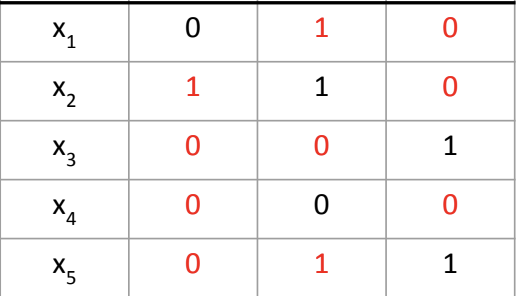
then we can use this model to directly estimate the reward for any action $a$ and context $x$, even the new policy is taking different actions against the logging policy.
$$V_{DM}(\pi) = \frac{1}{n} \sum_i \sum_a \pi(a|x_i) \times \widehat r(x_i,a) $$
where $n$ is total number of logging data we have.
Pros
- very low variance
Cons
- biased and not consistent (very terrible property, this means even we have infinite amount of logging data, we cannot accurately estimate the true value of new policy)
- potentially many hyper-parameters, because we need to train a regression model (which may also have a lot of hyper-parameters as well).
- because of the regression model $\hat r$, the evaluation is slow.
- it is in general very hard to get a accurate reward model in industrial recommend system
No assumption is made in this estimator.
Inverse Propensity Score (IPS)
Another method is to directly estimated the expectation via importance sampling. Specifically,
$$E_{p(x) \pi(a|x) q(r|x,a)}[r] = \int_x \int_a \int_r p(x) \pi(a|x) q(r|x,a) r dr da dx \\
= \int_x \int_a \int_r p(x) \pi(a|x) q(r|x,a) r \frac{\pi_0(a|x) }{\pi_0(a|x) } dr da dx \\
= \int_x \int_a \int_r p(x) \pi_0 (a|x) q(r|x,a) r \times \frac{\pi(a|x) }{\pi_0(a|x) } dr da dx \\
= E_{p(x) \pi_0 (a|x) q(r|x,a) } \left [\frac{\pi(a|x) }{\pi_0(a|x) } r \right] $$
Because we already have samples (the log data) drawn from joint distribution $p(x) \pi_0 (a|x) q(r|x,a)$, we can estimate the expectation using Monte-Carlo method and this will give us the formula of IPS method as
$$
V_{IPS}(\pi) = \frac{1}{n} \sum_i \frac{\pi(a_i|x_i) }{\pi_0(a_i|x_i) } r_i
$$
where $w(a_i,x_i) = \frac{\pi(a_i|x_i) }{\pi_0(a_i|x_i) }$ is usually called the vanilla importance weight (i.e. the inverse propensity).
Intuitive Explanation
Let’s say for some certain customer $x_i$, the old policy chose action $a$ with probability $p$ and observed a reward $r=1$. Now the new policy comes and for the same customer $x_i$, it has probability $q=2p$ of choosing action $a$. This means we have double chance of recommending $a$ to $x_i$, and we would expect we can gain $2r$ reward in the long run.
Pros
- unbiased and consistent (very nice) !
- very fast to evaluate, only O(n) time, do not need to sum over action spaces.
- hyper-parameter free !
- you don’t need to save the full distribution over actions, you only need to save the probability of taking $a_i$ for $x_i$.
Cons
- high variance if low number of samples or large action spaces
- Spoiler Alert: the high variance mainly because the vanilla importance weight is not robust, almost all advanced research works on IPS based model-free methods focuses on how to derive robust estimation of this importance weight.
Assumptions
- need to satisfy the common support assumption (because of importance sampling), in other words, $\pi(a|x_i) >0 \rightarrow \pi_0(a|x_i) >0$.
Doubly Robust (DR)
The above two methods can be seen as two extremes (DM with high bias but low variance, IPS is low bias but high variance), doubly robust tries to combine them into a single estimator to achieve low bias and low variances.
The key idea is to use the IPS method to correct the error of predict reward from DM method. In other words, we use the idea of IPS to estimate the expected difference of true reward against the predict reward, the formula is given as follows
$$
V_{DR}(\pi) = \frac{1}{n} \sum_i \sum_a \pi(a|x_i) \widehat r(x_i,a) + \frac{1}{n} \sum_i \frac{\pi(a_i|x_i) }{\pi_0(a_i|x_i) } (r_i - \widehat r(x_i,a) )
$$
It mainly consists of two parts: (1) the estimation from DM method, and (2) the estimation of deviation $r_i - \widehat r(x_i,a)$ using the idea of IPS method.
Pros
- low bias and variance
- unbiased and consistent
- works well with small samples
Cons
- potentially many hyper-parameters (less sensitive compared to DM)
- slow to evaluate
- can still fail in challenge cases (you can think it combines the advantages of two methods, but also have weakness of both methods as well)
Assumption
- need to satisfy common support assumption as well
Self-Normalized IPS (SNIPS) and Clip IPS (CIPS)
SNIPS is an improved version of IPS method and it is widely used by industrial practitioners because it is very simple and hyper-parameter free, and can also have very good performance (close to doubly robust) when the action space is small.
Recall that the main problem of IPS method is the variance can be very high. This is because that, for the vanilla sampling weight $w(a_i,x_i) = \frac{\pi(a_i|x_i) }{\pi_0(a_i|x_i) }$, it can be way too large if the logging policy $\pi_0$ has very little probability to conduct the action $a$. This phenomenon is even serious in the case of large action space.
One possible approach (Called Clip IPS) is to cut-off the importance weight that are too large, i.e.,
$$
w’(a_i,x_i) = \min \left ( \frac{\pi(a_i|x_i) }{\pi_0(a_i|x_i) } , \lambda\right)
$$
where $\lambda$ is the upper bound on the weight. Although appealing and simple, this method is biased and not consistent, and it introduce an extra hyper parameter to tune, which is hard to deal with in practice.
SNIPS avoid the potential large weights by normalize each weights respect to their own average, specifically, the importance weight is now
$$
w_s = w(a_i,x_i) / \frac{1}{n} \sum_i w(a_i,x_i)
$$
and we will have the SNIPS estimator as
$$
V_{SNIPS} (\pi) = \frac{1}{n} \sum_i w_s(a_i, x_i) r_i = \frac{\sum_i w(x_i, a_i) r_i}{ \sum_i w(x_i,a_i)}
$$
Another way to think about this is, instead of dividing by the sample number $n$, the denominator now becomes the sum of all importance weights. (A difference way of estimate weighted average).
Pros
- low bias, biased but consistent (still favorable)
- relatively low variance
- works very well when the number of actions is small
- parameter-free and very fast in practice
Cons
- not good in challenge case (small sample, large action space, etc.)
Assumption
- the same common support assumption
Why Large Action Space is Hard
With large action space, it is very easy to encounter the challenge problems, some of the cases may include:
- In the logging data, the policy $\pi_0$ may only conducted a small subset of actions, which make it very hard to estimate the distribution for logging policy over all actions. This will also cause the estimation the performance of new policy to be highly inaccurate, because the new policy can have high probability conduct a action that is never appeared in the logging for any context.
- It is more likely the new policy $\pi$ is heavily deviated from the original policy $\pi_0$. This is because that for large action space, typically the distribution over action can have long tail (in other words, most of probability mass is concentrated small amount of actions.) In such a case, if the user interacted with something new, the new policy might be quite different from the original, make it challenging .
- It also increase the time for evaluation, especially for direct method based estimators (need to collect more data).
Summary on Recent Estimators (by Jul. 2023)
In this section, I present some latest research works related to OPE estimators in large action space with a focus on IPS variants (model-free methods) because it is usually more practical and easier to use in industrial.
Each section title is associated with corresponding paper. if you are interested, you can check the original paper for more details.
Doubly Robust optimal shrinkage (DRos)
One of the issues with DR method is that, when comes to challenge settings where the new policy $\pi$ is highly different from the logging policy $\pi_0$, then almost all previous mentioned IPS based method (including DR because it uses IPS idea to correct bias) will fail and DM will be the best in such cases.
It is easy to see that IPS methods fails because that the values of importance weight $w(x_i, a_i)$ can be very different if $\pi$ deviates a lot from $\pi_0$. DRos approach tries to derive a different way of estimating the weight by introducing an extra hyper-parameter $\lambda$ and minimize a MSE upper bound. The detailed theory is somewhat complicated and you can check it here in the original paper (section 3.1). Here I will show the final formula for the estimator and it is very similar to DR method where only the estimation of importance weight is changed.
$$
V_{DRos}(\pi) = \frac{1}{n} \sum_i \sum_a \pi(a|x_i) \hat r(x_i,a) + \frac{1}{n} \sum_i \frac{ \lambda w(x_i, a_i)}{\lambda + w(x_i,a_i) ^2} (r_i - \widehat r(x_i,a) )
$$
Pro
- Works well with small amount of data
- Good performance in the challenge setting
Cons
- biased and inconsistent, but still very useful in challenge settings.
- Many hyper-parameters: $\lambda$ and the reward model $\widehat r$
- slow to evaluate as well
No assumptions needed, because now the denominator can never be zero.
SubGaussian IPS
Recall that the IPS method have very high variance because the vanilla importance weight can be really large when the evaluation policy (new policy) distribution is heavily deviated from the logging policy. SNIPS and CIPS try to resolve this problem through self-normalization and hard threshing. This work aims to solve this high weight problem through the notion of power mean.
Given the vanilla importance weight $w(a_i,x_i) = \frac{\pi(a_i|x_i) }{\pi_0(a_i|x_i) }$, we can define a $\lambda ,s$-corrected importance weight as
$$
w_{\lambda,s}(a,x) = \left[ \lambda + (1- \lambda) * w(a,x) ^ s \right] ^ {\frac{1}{s}}
$$
It can be treated as the weighted power mean between $w(a,x)$ and constant $1$, where the weights are controlled by $\lambda$.
By manually set $s=1$, we get the formula
$$
w_{SG}(a,x) = \frac{w(a,x)}{ \lambda * w(a,x) + 1-\lambda }
$$
By plugging this estimation of importance weight into IPS, we get Sub-Gaussian IPS as
$$
V_{SG-IPS} (\pi) = \frac{1}{n} \sum_i \frac{w(a,x)}{ \lambda * w(a,x) + 1-\lambda } r_i
$$
Note that we can also have self-normalization version of this estimator and the derivation is almost same just as SNIPS.
Pros
- More robust and lower variance compared to IPS.
- The bias is no longer unbiased (not sure if it is consistent, no proof is given by the authors).
- the hyper-parameter $\lambda$ has real meaning, this is the confidence you believe that new policy should have exact same expected reward as old policy.
Cons
- an extra parameters introduced.
No assumption is made in this estimator
Marginal IPS (MIPS)
This is one of the latest works that aim to develop accurate estimators for large action space. The main idea of this work is to make use of some extra information produced when some action is executed by the recommendation system.
For example, when the some furniture is recommended (usually through product id, this is one action), we can also get the type, color, size of this furniture. This is called the action embedding $e$ by the authors, and it let us to rethink the recommendation system in the following way: instead of thinking the recommendation system conducted the action recommended a furniture with certain id, we can think it recommended a furniture with certain type and color.
With this idea in mind, we might be able to use action embedding as a surrogate for actions, and develop a more robust estimator that make use the of the extra information about actions.
The following understanding may not be true after careful reading.
the assumption behind this is that, compared to the number of actions, the different combinations of action embedding is small, which will lead us a more robust estimator even if the action is very large.
This understanding is may not be true in practice, we can easily have multiple categorical variable that have a lot of possible values. In addition, we may also continuous variables in our action embedding.
One very important intuition behind this approach is that, the action embedding allows us to somehow evaluate the similarity and correlation between actions.
Reformulate the Data Generation Process
Since we assume there is action embedding $e$ available in our data, the author reformulated the data generation process as follows:
- we observe some contextual information (user profile) $x_i \sim p(x)$, where distribution $p$ is unknown to us.
- the policy $\pi_0$ take an action $a_i \sim \pi_0(a|x_i)$.
- we observe some action embedding $e_i \sim p(e|x_i,a_i)$, this distribution is unknown as well.
- we observe a reward $r_i \sim q(r|x_i,a_i,e_i)$, the distribution $q$ is unknown.
Because of the Therefore, under this data generation process, the logging data can be treated as
$$
{ x_i, a_i, e_i, r_i}_{i=1}^n
$$
Now, the OPE problem can be formulated as
$$V(\pi) = E_{p(x) \pi(a|x) p(e|x,a) q(r|x,a,e)} \hspace{4pt} [r]$$
It seems that the problem becomes more complicated after introducing extra variables but actually it can be simplified with appropriate assumption. Specifically, the author made an assumption called no direct effect from $a$ to $r$. In other words, the uncertainty of reward $r$ should be fully explained by just user profile $x$ and the action embedding $e$, statistically, this means $r \perp a | x,e$.
Taking our previous example, it basically assumes that whether the customer will buy (or click) our furniture is only depend the type and color of a furniture, not some specific product. Note that in practice, we can have better and more action embedding, but you can see that this assumption is usually not true in practice.
Nevertheless, with this assumption, we can derive the MIPS estimators as follows
$$
E_{p(x) \pi(a|x) p(e|x,a) q(r|x,a,e)} \hspace{4pt} [r] \\
= E_{p(x) \pi(a|x) p(e|x,a) q(r|x,e)} \hspace{4pt} [r]
= E_{p(x) p(e|x,\pi) q(r|x,e)} \hspace{4pt} [r] \\
= E_{p(x) p(e|x,\pi_0) q(r|x,e)} \hspace{4pt} \left [r \frac{p(e|x,\pi)}{p(e|x,\pi_0)} \right ]
$$
where $p(e|x,\pi) = \sum_a \pi(a|x) p(e|x,a)$ is the marginal distribution. From the first step to second step, we use the assumption and sum out action $a$ (only two terms involved after using the assumption) to get a new conditional distribution over just $e$. From the second step to third step, we use the same trick of deriving IPS formula.
Bias and Variance Trade-Off
As mentioned before, the assumption made by the authors can never be fully true in practice. However, this won’t limit the practical use of this estimator as the authors find.
If this assumption is fully satisfied (no bias in this case), then it is very likely that the embedding space is large as well, and thus incurs a lot of variances.
If this assumption is violated, the variance decrease and bias would increase as well.
The best performance achieved when we deliberately violate the assumption to some extent (i.e. determine the number and which features should be considered in embedding space).
Practical Implementation Concerns
Calculate $w(x,e) = \frac{p(e|x,\pi)}{p(e|x,\pi_0)}$ is typically very hard in practice, this is because we don’t know the distribution $p(e|a,x)$ and we can only estimate through the data. But in fact, estimate this distribution through data is also very hard, because there might be multiple variables in $e$ and it can be continuous or categorical, the joint space over the $e$ is very large and hard to regression onto in practice.
The authors provided an alternative way to estimate this value through the Bayes rule.
$$
w(x,e) = \sum_a \pi_0(a|x,e) \frac{\pi(a|x)}{\pi_0(a|x)} =E_{\pi_0(a|x,e)} [w(x,a)]
$$
The detailed derivation is shown here (this proof is located at page 19 of the original paper.).
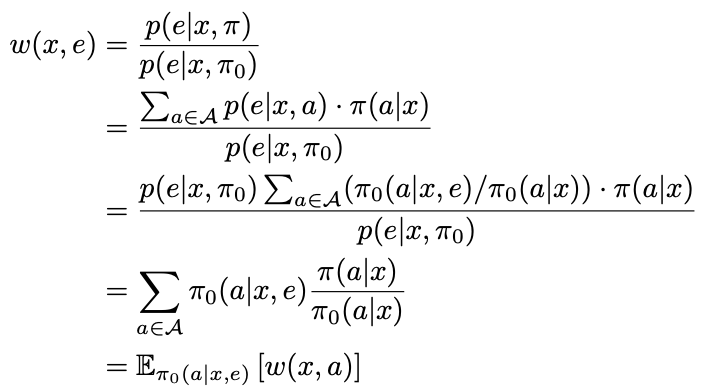
where $w(x,a) = \frac{\pi(x|a)} {\pi_0(x|a)}$ is the vanilla importance weight. In addition, from step 2 to 3, the following formula is used for transformation.
$$
p(e|x,a) = \frac{\pi_0(a|x,e) p(e|x,\pi_0)}{\pi_0(a|x)}
$$
With this new way of calculating of $w(x,e)$, what we need is to estimate $\pi_0(a|x,e)$. Because action is nothing but a single categorical variable which can take multiple values, this is relatively easy to do with an regression model in most cases (e.g. Logistic Regression, or any other model can output distribution over labels), with customer features and embedding features as input.
You may want to use very complicated model such as deep neural network (with soft max layer at the end) for this regression problem. However, from my personal understanding, a simple regression model is usually preferred in this case.
To understand why, we need to have a better understanding of the relationship between action $a$ and embedding $e$. Specially, in practice, once the action $a$ is determined, $e$ will be determined as well (think the product recommendation example, the color, type, size of given a product id is determined).
Now let’s consider the reverse, if the embedding $e$ is given, can we uniquely identify the action $a$ ? The answer is yes when the assumption is true, and no otherwise. However, in practice, if there is continuous variable present in the embedding, this is usually true as well (e.g. there will be little chance that two same objects have exact same size).
This is not a typical learning problem where the we will have different values of some features but have the same label. In our case, if label is the same, then the embedding feature is exactly same as well.
So what are we doing here? Given some features that determines the action to predict the action ?
the following is just my own intuitive understanding, nothing to do what stated in the original paper.
It is true we can predict the action exactly, but only when we have a very sophisticated model such as a very deep neural work or a decision tree with unlimited depth. In this case, the output distribution over action put all mass into the target action, which is not we want (falls back to previous vanilla importance weight).
This is why I conclude that a slightly simpler model is preferred here. A linear model such as logistic regression won’t have the ability to remember input cases and distinguish between the minor difference between continuous values. Instead, because the limited ability, it will distribute the whole probability mass 1.0 over all action that have similar action embedding as the one of target action, and this distribution is used to smooth the vanilla importance sampling weight, make it more robust.
Discussion over this understanding is welcome (by Leon).
Pros
- low variance and unbiased when the assumption is true
- Good performance in large action space, can beat Direct Method, and it converges fast.
- Good practical performance even if the assumption is break
- We can have self-normalized version of MIPS as well.
Cons
- need extra feature in your data, i.e. the action embeddings
- Need to determine the number of features and which feature (action embedding) you want to use, just like the hyper-parameter search
- Slow evaluation speed because now you need to sum over the action space.
- need to train a regression model over the action space
- need to save the distribution over all actions for single context $x_i$. If action space is large (e.g. 5000), we essentially need 5k times the memory.
Assumption
- It has the no direct impact assumption, in other words, give the action embedding $e$ and user profile $x$, the reward $r$ is independent of $a$, i.e., $r \perp a | x,e$. More action embedding features, more likely the above assumption is true. But too many features can greatly increase the variance as well (it basically falls back to vanilla weight cases where there might be large number of different combination of action embedding $e$).
- Common embedding support assumption.
Learned-MIPS (AutoMIPS)
As discussed in the above section, although the no direct impact assumption can hardly be satisfied in practice, it won’t affect the practical performance of the MIPS estimator. The major issue is that we may not have any action embedding features or the action embedding is too bad or too little (if too many, we can always use part of them).
So can we learn the action embedding through data directly? The answer is Yes, and it actually work pretty like a direct method.
So our goal is find some embedding $e$ that can be served as surrogate for action $a$. Specifically, the author assumes that there exist embedding $e \in R^d$ for each action $a$, such that $p(r|x,e) \approx p(r|x,a)$, for every context. This assumption is very similar to the previous one, but is more stronger where we also assumes that give action $a$, the reward is also independent of embedding $e$ as well.
Design Heuristics and Algorithms
The idea authors used through out the paper is that if $e$ is a very good representation of $a$, then it should be able to used to estimated the reward model very well.
Mathematically, we want to learn a function $f$ that take action $a$ as input and output the embedding $e = f(a)$, such that
$$
\sum_i \left ( r_i - G(x_i, e = f(a_i)) \right ) ^2
$$
is minimized. Where $G$ is the reward model to estimate the rewards (this is basically what we did in direct method). After this model is trained, we can simply use function $f$ the generate the action embedding for all action we have.
For example, in the paper, the author use a linear layer with input dimension $u = |A|$ (number of actions) and output dimension $v$ (the number of customer features) as the function $f$ (parameter size $W_{u \times v}$) and $\widehat r = G(x,f(a)) = x^Tf(a)$. Note that the input $a$ is in the one hot representation.
Side note, we can have bias parameter in the dot product as well. By append a constant 1 to all $x$ and increase the output dimension as $v+1$.
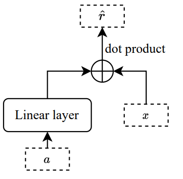
From a different view, because the input is one hot, when we use this linear layer as a function to generate our action embedding, it basically spit out one of the rows of its weight matrix $W_{u \times v}$. Therefore, we can think that, for each action $a_i$, we fitted a linear model with parameters $W_{i,\cdot }$ which take $x$ as input and try to predict the reward $r$. This allow us to think this whole framework of learning from a different point of view.
Again, we can see that action determines embedding, and it is almost true that the embedding determines actions as well. It almost impossible to have two exact same rows in the weight matrix $W_{u \times v}$.
Recall that for reward model $p(r|x,a)$, we know that if action $a$ is fixed, then r only depends $x$, so if we can train a model $r = G_{\theta}(x)$ where $\theta$ is the parameters, then we can use $\theta$ as the action embedding for $a$.
Once the action embedding is generated, we can use it in MIPS for estimation.
This estimator is an extension of MIPS, so I think it share similar pro and cons as MIPS, so details are omitted here.
Practical Concern
Because we need train a model that takes $x$ to predict $r$ for each action, the number of parameters in this model must be great than the dimension of $x$ (unless you only use partial information from x, which is a waste of computation and information).
In this case, how can we learn action embedding that is of arbitrary size. The solution I came up with is to train an encoder jointly with these linear models. Because the encoder parameters are same for all actions, we don’t need to contain them in our action embedding.
Group-IPS
Because we have the action embedding, and it can be used to estimator and similarity and relation between the actions. Why not do clustering over the action embedding space and group similar action together? In such way, we can significantly reduce the number of actions and then we can directly use IPS or SNIPS for estimation.
Specifically, let’s say we divided the whole action space $A$ into $k$ groups $g_1, …g_k$. Then for each logging row $(x_i, a_i, r_i)$, we change into $(x_i, g_i, r_i)$ where $a_i \in g_i$. Then the importance weight becomes
$$
w(g_i, x_i) = \frac{\pi(g_i|x_i)}{\pi_0(g_i | x_i)}
$$
where $\pi(g_i|x_i) = \sum_{a \in g_i} \pi(a|x_i)$.
Here, we can treat $g_i$ as the surrogate action and we transform our distribution over original action space $a$ into group space $g$, and then we can directly apply IPS or SNIPS for estimation.
Balanced IPS
Balanced IPS replace the vanilla importance sampling weight with a density ratio estimation using classifiers, it works as follows.
Let’s say we have a new policy $\pi$, thus given any context $x_i$, we can generate an action $a_i$ from $\pi(a|x_i)$, and we can mark this pair with label $C = 1$, i.e. ${x_i,a_i,1}$. We also have a lot of ${x_i,a_i,r_i}$ pairs from the logging policy, we extract the context and action from them and mark these pairs with label $C=0$ as ${x_i,a_i,0}$.
With these data, we can train a model that takes $x$ and $a$ as input and output a distribution over labels (0,1). This means we train a classifier to predict $p_0 = p(0|x,a)$ and $p_1 = p(1|x,a) = 1 - p(0|x,a)$.
Then we can estimate the importance weight as
$$
\frac{\pi(x,a)}{\pi_0(x,a)}
= \frac{p(x,a|C=1)p(C=1)}{p(x,a|C=0) p( C=0)}
= \frac{p(C=1|x,a)}{p(C=0|x,a)}
= \frac{p_1}{p_0}
$$
where $P(C=1) = P(C=0)$ by picking same amount of training samples from both policy, with this design, we can get the formula of Balanced IPS as
$$
V_{B-IPS} (\pi) = \frac{1}{n} \sum_i \frac{p_1}{p_0} r_i
$$
where $p_1$ anad $p_0$ is the probabilities we get the from the classification model.
Improvement
The original BIPS uses action itself to train the model. Because action is usually the categorical variable and there is no relation between each of them. I proposed to use action embedding to train the classification model and it can significantly boost the performance of BIPS.
Evaluation of Estimators (Meta-Evaluation)
Our task of meta evaluation is to estimate the bias and variance of each estimators under large action space cases through simulation experiments.
To this end, we need the following components and data:
- the action space should be large
- the old policy $\pi_0$ (usually the policy that already been put into production)
- the logging data generated by the old policy $D_0$.
- the new policy $\pi$
- the A/B test/logging data of new policy $D$.
Note that we won’t have the logging data for the policy we are currently developing in practice. In such cases, we can treat the new policy as current policy in production, and the old policy as the previous policy just before that one, which enables us to conduct meta-evaluation of estimators.
Steps
In order to estimate the bias and variance of an estimator (e.g. snips), we can follow these steps.
Compute the true policy value (the expectation of reward) $v_{\pi}$ of the new policy $\pi$ . this is usually estimated using its own logging data $D$, we treat this estimation as the true value (this is the best we can do, unless we have infinite number of logging data or we know the true distribution of context and reward model).
Build $N$ bootstrap dataset $D_0^i, i = 1..N$ from the dataset $D_0$, which is the logging dataset generated by the old policy.
For each estimator, using the bootstrap dataset $D_0^i, i = 1..N$ to estimate the expected reward of new policy $N$ times, and now we would have $N$ different estimation of this estimator. Based on these values, we can estimate the bias, variance and MSE as usual.
Repeat for all estimators being tested.