Support Vector Machines (SVMs) stand out as an exceptionally elegant model that has captivated me over the years. Although it is not widely employed after the advent of neural networks, it still plays an important part in machine learning, such as in cases with limited data.

I have studied the SVM model for over four years and still find myself fascinated by the theory behind it. In this post, I will delve into the theoretical foundations of SVM, coupled with practical implementation. I will begin with the naive SVM in primal space, and then extend to slack SVM. After that, we will talk about SVM in dual space and introduce the kernel trick that makes SVM an incredibly powerful model in practice.

Motivation and Formulation

Linear classifiers such as Perceptron have been widely employed, but one of the disadvantages is that it cannot distinguish between two lines (or decision boundaries) if they can both perfectly separate the input data.

Specifically, as shown in the following figure, both line A and B are the same from the perspective of Perceptron. However, we usually believe that B is a better decision boundary because it is further “away” from the training data points. This means B generalize better than A and is usually more robust in practice. For example, if we add some noise to the data, model A can change its prediction easier compared to model B.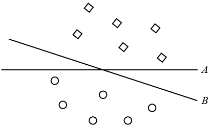

SVM is developed with this idea of “max margin” in mind. Specifically, as shown in the following figure, SVM tries to find a decision hyper plane $w^T x +b = 0$ such that

1. for all positive training instances (square in the figure, with label $y^{(i)}$ = 1), we have $w^T x^{(i)} + b >= c$
2. for all negative training instances (circle in the figure, with label $y^{(i)}$ = -1), we have $w^T x^{(i)} + b <= -c$

where the $\{x^{(i)}, y^{(i)} \}$ here denotes the $i^{th}$ input training instance.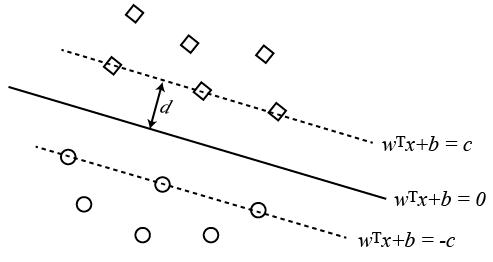

In Perceptron, we only care about the sign (which side). But in SVM, we care not only the sign, but also the distance to the decision boundary, which is also called the margin.

The objective of SVM is to maximize the margin, as indicated by the distance between these parallel lines (i.e., the $d$ in the figure). To calculate the distance $d$, we arbitrarily pick two points $p,q$ on the line $w^T x + b = c$ and $w^T x + b = 0$, respectively.

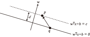
Then, because the vector $w$ is perpendicular to the hyper plane, the projection of the vector $p-q$ on $w$ would have its norm equal to $d$, i.e.
$$
d = \frac{ w \cdot (p-q)}{\lVert w \rVert} = \frac{w^T p + b - w^T q - b}{\lVert w \rVert} = \frac{c}{\lVert w \rVert}
$$

Note that there will be only one line that achieves the maximum margin. However, this does NOT mean there is only one unique solution to the parameters $w,b,c$. In fact, if $w,b,c$ solves the problem, then $kw, kb, kc$ is also a valid solution for any $k \ne 0$. Therefore, without loss of generality and by the property of scale invariant, we manually set $c = 1$.

With all of the analysis above, the optimization problem of SVM can be formulated as
$$
\min_{w,b} \quad \frac{1}{2} \lVert w \rVert ^ 2 \\
s.t. \quad y^{(i)} (w^T x^{(i)}+b) \ge 1, \forall i
$$

Note that the original objective function $\max \frac{1}{\lVert w \rVert}$ is replaced with an equivalent objective function $\min \frac{1}{2} \lVert w \rVert ^ 2$ for the ease of optimization. In fact, the above problem is a Quadratic Programming problem and can be solved using existing solvers such as quadprog in MATLAB or cvxopt in Python. And we will talk about the implementation in detail in the later sections.

Limitations of Naive SVM

The naive SVM is formulated under the assumption that data is separable. However, this is rarely the cases in practice, and there are two commonly employed approaches to tackle this issue. What’s more, you can combine the following two methods and use them together when developing the SVM on real-world dataset.

Slack SVM

The first approach make use the idea of slackness. To be more specific, for each data instances in the training set, we introduce a new parameter $\xi_i$ to denote the amount of violation allowed in the constraint. In other words, we replace the constraint
$$
y^{(i)} (w^T x^{(i)}+b) \ge 1, \forall i
$$
with
$$
y^{(i)} (w^T x^{(i)}+b) \ge 1 - \xi_i, \forall i \\
\xi_i \ge 0, \forall i
$$

In addition, we penalize each of the violations in the new objective function as follows.
$$
\min_{w,b, \xi_i} \quad \frac{1}{2} \lVert w \rVert ^ 2 + \lambda \sum_i \xi_i
$$
The hyper parameter $\lambda$ here denotes the amount of penalty we have to pay for each unit violation of constraints. With all the modifications discussed above, the soft slack SVM problem is
$$
\min_{w,b, \xi_i} \quad \frac{1}{2} \lVert w \rVert ^ 2 + \lambda \sum_i \xi_i \\
s.t. \quad y^{(i)} (w^T x^{(i)}+b) \ge 1 - \xi_i, \forall i \\
\quad \xi_i \ge 0, \forall i
$$

The above optimization problem is also in the Quadratic Programming (QP) form and therefore can be solved in the same way as the naive SVM. In addition, due to the extra $\xi_i$ parameters, we can transform this problem in to an unconstrained optimization problem. This is because that when we reach the optimal solution, the value of $\xi_i$ must be
$$
\xi_i = \max \{ 0, 1- y^{(i)} (w^T x^{(i)} +b) \}
$$
This is also known as the hinge loss (or max-margin) loss of SVM.

Here is the proof sketch of the above conclusion. We denote $D_i = y^{(i)} (w^T x^{(i)} +b)$.

• If we already have $D_i \ge 1$ for the optimal $w,b$, then $\xi_i$ must be zero in order to minimize the objective.
• Otherwise, we would have $D_i < 1$, and in order to satisfy the constraint, we must have $\xi_i \ge 1-D_i$. Because the objective penalize larger $\xi_i$, therefore the optimal value for $\xi_i$ must be $1-D_i$.

With this key observation, we can plug this equation back into the objective and we will now have an unconstrained optimization problem as follows.
$$
\min_{w,b} \quad \frac{1}{2} \lVert w \rVert ^ 2 + \lambda \sum_i \max \{ 0, 1- y^{(i)} (w^T x^{(i)} +b) \}
$$
And this problem can be solved easily using gradient based methods such as stochastic gradient descent (SGD). Note that the parameter $\xi_i$ is gone in this formulation.

One side note is that, when we have imbalanced data, we can modify the objective function to account for the data imbalance in the case of SVM. For example, we can modify the objective function as
$$
\min_{w,b, \xi_i} \quad \frac{1}{2} \lVert w \rVert ^ 2 + \lambda \left( \frac{N_{-1}}{N} \sum_{i, y^{(i)} = 1} \xi_i + \frac{N_{1}}{N} \sum_{i, y^{(i)} = -1} \xi_i \right)
$$
where $N_{-1}, N_{1}, N$ denotes the number of negative, positive and total training instances. If we have much more negative instances (i.e. $N_{1} \ll N_{-1}$), the penalty we pay for the negative instances is low while the penalty for positive instances is high. Therefore, the model will pay more attention to positive example and try to classify all of them right with large enough distance to the decision boundary.

Data Feature Mapping

Another approach to overcome the separable assumption is to employ a feature mapping function $\phi(x)$, such that the data becomes linear separable after mapping all the training data into the feature space.

For example, assume we have a set of 2D points $x^{(i)} = (x^{(i)}_1,x^{(i)}_2)$ that are not linear separable in the original space. One example feature mapping we can use here is
$$
\phi(x^{(i)}) = (x_1^{(i)} x_1^{(i)}, x_2^{(i)} x_2^{(i)} , x_1^{(i)} x_2^{(i)})
$$
, and fitting a linear decision plane in the feature space would correspond to fitting a second-order polynomial in original space, which helps separating the data.

We can see that $w^T \phi(x) +b = w_1 x_1^2 + w_2 x_2^2 + w_3 x_1 x_2 + b$, which corresponds the geometry equation of second order polynomial in the original space.

Although simple and appealing, one biggest disadvantage is that data feature mapping usually increase the dimension of input data, make the whole optimization problem more complex and increase the time for solving the Quadratic programming (the size of $w$ increase). In addition, it also increase the inference time because we have to apply the feature mapping to the input data first. This issue can be quite significant if we are using high order of polynomial feature mapping.

Implementation of SVM

Although there are already quadratic programming solvers, apply them to solve the optimization problem in SVM is not a trivial task. In this section, I will walk you through the process of reformatting the optimization problem of slack SVM into the standard form required by the standard quadratic programming solver. Note that different solvers may have slightly different standard form, and for this blog post, I will mainly focus on the cvxopt solver in Python.

From the official API document of quadratic programming in cvxopt, we can see that the standard form is
$$
\min_{x} \frac{1}{2} x^T P x + q^T x \\
s.t. \quad Gx \le h, \quad Ax = b
$$
while the formulation of slack SVM is
$$
\min_{w,b, \xi_i} \quad \frac{1}{2} \lVert w \rVert ^ 2 + \lambda \sum_i \xi_i \\
s.t. \quad y^{(i)} (w^T x^{(i)}+b) \ge 1 - \xi_i, \forall i \\
\quad \xi_i \ge 0, \forall i
$$

Because we don’t have equality constraints in our case, therefore we just need to find $P, q, G, h$ and pass these matrix as the arguments for the solver.

Let’s assume we have $N$ training instances with $F$ features, then the total number of unknown parameters $x$ here is of size $K = F+1+N$, i.e.
$$
x = [w_1,…,w_F,b,\xi_1,…, \xi_N]^T
$$

The first thing we need to figure out is the value of $P_{K \times K}$ and $q_{K \times 1}$, such that
$$
\frac{1}{2} x^T P x = \frac{1}{2} \lVert w \rVert ^ 2, \quad q^T x = \lambda \sum_i \xi_i
$$

From the first equation, because $\lVert w \rVert ^ 2 = w_1^2 + … + w_F^2$, we can set $P_{K \times K}$ as
$$
\begin{bmatrix}
I_F & 0 \\
0 & 0
\end{bmatrix}
$$

where $I_F$ is the identity matrix of size $F \times F$. From the second equation, we can easily see that
$$
q_{K \times 1} = [0_{1 \times F}, 0, \lambda_{1 \times N}] ^ T
$$

Now we have found the coefficient matrix $P,q$, and the next two matrix to figure out is $G,h$. First, let’s figure out the size of these two matrix. From the formulation of slack SVM, we can see that we have two types of inequality constraints and each of them have $N$ constraints inside. Therefore, the total number of inequality constrains is $2N$, and the size of $G,h$ is $2N \times K$ and $2N \times 1$, respectively.

For matrix $G$, the upper half should represent the constraint $y^{(i)} (w^T x^{(i)}+b) \ge 1 - \xi_i$, for a more clear looking at the coefficient, we can transform it into
$$
-y^{(i)} (x^{(i)})^T w - y^{(i)} b - \xi_i \le -1
$$

Therefore, we can conclude the upper half of $G,h$ as
$$
G_u =\left [ [-y^{(i)} (x^{(i)})^T] _{N \times F}, [- y^{(i)}] _{N \times 1}, - I _N \right] \\
h_u = [-1_{N \times 1}]
$$

For the bottom half of the matrix $G,h$, it corresponds to constraint $- \xi_i \le 0$, and we can easily find
$$
G_b = [0_{N \times F}, 0_{N \times 1}, - I_N] \\
h_b = [0_{N \times 1}]
$$

Finally, we just need to stack the up and bottom half of these two matrix.

Python Code

With the above analysis, in the implementation phase, what we need to do is just create these four matrix based on the given data. However, because the for loop in python is extremely slow, we need to make use of vectorized operations in numpy to construct these matrix. One example of Python implementation is shown as follows.

1
2
3
4
5
6
7
8
9
10
11
12
13
14
15
16
17
18
19
20
21
22
23
24
25
26
27
28
29
30
31
32
33
34
35
36
37
38
39
40
41
42
43
44
45
46
47
48
49
50
51
52

import numpy as np
from cvxopt import solvers,matrix

class SlackSVM:
    def __init__(self, lmda):
        self.lmda = lmda

    def fit(self, X, y):
        # X is a 2D array with shape N x F
        # y is a 1D array with size N, contains only {1, -1}

        N, F = X.shape
        assert(N == y.size), 'Wrong input, size mismatch!'
        n_paras = F+1+N
        # construct P
        P = np.zeros(n_paras)
        P[:F] = 1
        P = np.diag(P)

        # construct q
        q = np.zeros(n_paras)
        q[F+1:] = self.lmda

        # construct G upper
        G = np.zeros( shape = (N<<1 , n_paras) )
        y_r = y.reshape(N,1)
        G[:N, :F] = -y_r * X # numpy auto broadcasting
        G[:N, F:(F+1)] = -y_r
        G[:N, F+1:] = -np.identity(N)
        # construct G bottom
        G[N:, F+1:] = -np.identity(N)

        # construct h
        h = np.zeros( N<<1 )
        h[:N] = -1

        # call solver
        ret = solvers.qp(matrix(P),matrix(q),matrix(G),matrix(h))
        solution = np.array(ret['x']).flatten()

        # extract w,b from solution
        W = solution[0:F].reshape(F,1)
        b = solution[F]

        self.W  = W
        self.b = b
        return self

    def predict(self, X):
        # X should be a 2D array of size N x F
        preds = (X @ self.W + self.b).flatten()
        return np.where(preds > 0, 1, -1)

The above implementation is in scikit-learn style, and we can define and train the SVM model using the similar syntax like other models in scikit-learn.

In addition, there are some other things in the implementation that are worth noting:

1. the input to the qp solver must be of matrix type defined in cvxopt, not numpy.ndarray. Therefore, we need to convert these matrix before passing into the solver.
2. the n_paras is the $K$ we used in the above analysis.
3. the values of $\xi_i$ is not important during the prediction time, and therefore we don’t save it.
4. the input is assume to be cleaned with label {-1, 1}.

This concludes the first part of my comprehensive guide towards support vector machines. In the future posts, I will talk about Lagrange Duality as well as the dual SVM, and how kernel metric can be applied.

• ← Previous Post
• Next Post →